January
How can an external file be deleted using SAS? One way is to use the 'X' command and use a system command like 'DEL' in DOS. But another way is to use the FDELETE function inside a datastep as the following example demonstrates:
   data _null_;

      ** Assign the external file being deleted to a reference 'fn' using
         the FILENAME statement;
      rc=FILENAME('fn',"c:\temp\dmext.txt");

      ** Now delete the file using the FDELETE statement -- if RC does
         not equal zero then there is an issue;
      rc=FDELETE('fn');
      if rc=0 then put "File deleted";
      else put "ERR" "OR: Issue with trying to delete the file";

      ** Clear the FILENAME reference 'fn';
      rc=FILENAME('fn');

   run;
In the example the dataset DMEXT.TXT in the directory C:\TEMP is deleted -- there is also an additional piece of code that puts out a message as to whether there is an issue with the deleting of the file or not.
Hope this helps. Have a very good 2010.
February
I recently had a question from Bob in New Jersey asking me to look at whether NODUPKEY always selected the first record in a BY group -- his opinion was that it always did.
The short answer is 'NOT REALLY'. However the answer does depend on two other options -- the EQUALS|NOEQUALS option in the SORT procedure, and the global option SORTEQUAL|NOSORTEQUALS (default when shipped from SAS is SORTEQUAL).
Lets look at first what the global option SORTEQUAL|NOSORTEQUALS is all about, quoting from the SAS documentation:
The global option SORTEQUAL|NOSORTEQUALS dictates if the EQUALS or NOEQUALS option is set by default in the SORT procedure, where:
SORTEQUALS
specifies that observations with identical BY variable values are to retain the same relative positions in the output data set as in the input data set.NOSORTEQUALS
specifies that no resources be used to control the order of observations with identical BY variable values in the output data set.
It is interesting to note that SAS suggests that in order to save resources, use NOSORTEQUALS when you do not need to maintain a specific order of observations with identical BY variable values.
Now lets look at the EQUALS|NOEQUALS option in the SORT procedure:
Specifies the order of the observations in the output data set. For observations with identical BY-variable values, EQUALS maintains the relative order of the observations within the input data set in the output data set. This is in contrast to the NOEQUALS that does not necessarily preserve this order in the output data set.
From the SAS documentation, the NOEQUALS option is useful if you are sorting a large dataset as it can save in CPU but has the disadvantage of producing inconsistent results in your output data sets if you run the code multiple times.
Now that we have looked at all the documentation, lets take a look at some data:
   data ae0;
      input ptnum $6. aeseq event $20.;
   cards;
   001002 1 HEADACHE
   001001 1 FEVER
   001001 2 HEADACHE
   001003 1 NAUSEA
   001003 4 DIARRHEOA
   001003 2 VOMITING
   001004 1 DIARRHEOA
   001001 3 DIARRHEOA
   001002 2 DIARRHEOA
   001004 2 HEADACHE
   001003 3 FEVER
   ;
   run;
In addition, to make sure the global option SORTEQUAL|NOSORTEQUALS is set to its usual shipped default the option shall be set to SORTEQUAL:
options SORTEQUAL;
Now lets look at the following code where we just use NODUPKEY (I have put the EQUALS option for clarity although this is not needed with the setting of the global option SORTEQUAL):
   proc sort data=ae0 out=ae1 nodupkey equals;
      by ptnum;
   title1 "Data with NODUPKEY and EQUALS";
   proc print data=ae1 noobs;
   run;

   === Output ===
   Data with NODUPKEY and EQUALS

   ptnum     aeseq    event

   001001      1      FEVER
   001002      1      HEADACHE
   001003      1      NAUSEA
   001004      1      DIARRHEOA
In the code above the first record of each "by group" value is output, i.e. the first record in the sequence. Now lets just suppose that the option EQUALS|NOEQUALS was set to NOEQUALS (or the setting of the global option NOSORTEQUALS):
   proc sort data=ae0 out=ae1 nodupkey noequals;
      by ptnum;
   title1 "Data with NODUPKEY and NOEQUALS";
   proc print data=ae1 noobs;
   run;

   === Output ===
   Data with NODUPKEY and NOEQUALS

   ptnum     aeseq    event

   001001      3      DIARRHEOA
   001002      1      HEADACHE
   001003      3      FEVER
   001004      1      DIARRHEOA
Note that the output shows that it is not necessarily the first record for the PTNUM variable.
Inside SAS there are a large number of SAS options that can affect the output that is produced, whether is be from a procedure or datastep. If your program produces unexpected results, after you have gone though looking at the SAS LOG and exhausted other remedies, take a look at the SAS options that are applied.
I know this is a very technical tip this month but I hope that it shows that SAS is a very sophisticated piece of software and must be treated with respect. I hope this topic is interesting for some. See you in March.
March
The DATASETS procedure has been around for a long time. Its main purpose is to manage your SAS datasets with tasks that include copying, deleting and renaming datasets, renaming variables inside a dataset, and adding formats and labels to a dataset. The procedure can also manage indexes inside a dataset. But one thing that is not clear is how to drop or keep variables in a dataset.
There is a little trick that is useful when you want to DROP or KEEP variables in a dataset -- use the APPEND statement, as the following statement shows:
   PROC DATASETS LIBRARY=work;

      ** Copy in the CLASS dataset from SASHELP;
      COPY IN=sashelp OUT=work;
         SELECT class;

      ** DROP variable AGE from the dataset;
      APPEND BASE=class0 DATA=class (DROP=age);

      QUIT;
   RUN;
In this example we have made a copy of the dataset CLASS and created CLASS0, on the way we have also dropped the variable AGE. Note that the BASE and DATA options in the APPEND statement are different -- you cannot have these two parameters with the same name (I personally believe this is a nice feature as it forces the programmer to create a new dataset with each step of a program, and makes the task of reading the program by another person easier). It also must be noted that the dataset CLASS0 must not exist -- if it does then any data in CLASS will be appended to CLASS0.
At first thought the COPY statement should do this task but this statement will not allow you to run the normal dataset options like the DROP and KEEP statements, only the APPEND procedure will allow you to this.
Hope you have a happy and safe March -- see you in April.
April
Sometimes in our program we want to get information from the option settings -- this can be something like LINESIZE information or the program name. The function that is useful to do this is the GETOPTION function.
The following code gets the LINESIZE option value and sets a horizontal line to a macro variable _horizonalLine to that length:
   data _null_;
      _lineSize=getoption('ls');
      _horizonalLine=repeat('_',_lineSize-1);
      call symput('_horizonalLine',strip(_horizonalLine));
   run;
In the example above, the number of '_'s in the horizontal line is set from the LINESIZE setting -- if there is a LINESIZE of 77 then there will be a horizontal line made with 77 '_'s.
Similarly, the program name can be set using the SYSIN option value (this is only available in Batch mode -- the value will be blank for interactive mode) as the following code demonstrates:
   data _null_;
      _pgmName=getoption('sysin');
      if missing(_pgmName) then _pgmname='Interactive';
      call symput('_pgmName',strip(_pgmName));
   run;
Please note that what comes out of the SYSIN value is host dependent as some times the program name and directory is given and other times it is the program name only -- try it on your system first.
The following code will print the CLASS dataset and add a footnote with a horizontal line and put the program name and date/time the program run (note that you must save the SAS program as a
   options nodate nonumber ls=77;
   run;
   data _null_;
      ** Get linesize and set a horizontal line;
      _lineSize=getoption('ls');
      _horizonalLine=repeat('_',_lineSize-1);
      call symput('_horizonalLine',strip(_horizonalLine));
      ** Get Program Name;
      _pgmName=getoption('sysin');
      if missing(_pgmName) then _pgmName='Interactive';
      call symput('_pgmName',strip(_pgmName));
   run;

   title1 'Listing of CLASS data';
   footnote1 "&_horizonalLine";
   footnote2 "Program Name: &_pgmName  Generation Date/Time: &sysdate9. &systime.";
   run;
   proc print data=sashelp.class;
   run;
Note the use of the double quotes around the text that contains the macro variables _horizonalLine and _pgmName -- as a general rule SAS will not resolve macro variable if single quotes are used.
This month is the start of conference season with SAS Global Forum starting in Seatle, WA on April 11 through April 14. If you cannot be there in person, please visit the Global SAS Forum web site and get updates -- there will be among other things a summary of the days' happenings and discussions from key people on the direction SAS is taking.
See you in May.
May
This month is a quick tip about appending data -- making a SAS datastep do what a APPEND statement or procedure call does.
First lets have a look at some data:
   data x;
      length a b d 8;
      call missing(of _all_);
      delete;
   run;
   data y;
      length a b c d 8;
      input a b c d;
   datalines;
   1 2 3 5
   2 3 6 4
   ;
   run;
The usual way of appending the data in dataset y to dataset x is to do the following:
   proc datasets library=work nolist nodetails nowarn;
      append base=x data=y force;
      quit;
   run;
But as I mentioned above, we do not want to use the APPEND statement so is there another way? Could be use the following:
   data x;
      set x y;
   run;
Using a datastep, the SET statement will not quite do it as the variables in datasets x and y are added to x, resulting in dataset x having variable c that is not in the initial datastep.
What must be considered is using a statement that will take the structure of dataset x, and then get the records of dataset y and apply them to dataset x without changing the structure, as the following will do:
   data x;
      if 0 then modify x;
      set y;
      output;
   run;
This has the effect of calling the dataset x in modify mode (therefore variables cannot be created in dataset x) and bringing in the data from y. The output statement outputs the record to dataset x.
Coming up later this month I will be presenting two papers at PharmaSUG in Orlando -- one will be a presentation doing a countdown of the Top Ten ways to Merge data, and a second is presenting a small macro that will turn an ASCII Text output to an RTF output inside a single datastep, with the use of ODS! If you are there, please come and say 'hi'.
June
While at PharmaSUG this year in Orlando, a person asked me for a way that SAS could generate a selection of integers from 1 to 10 inclusive. When we looked around quickly on the web nothing could be found so I thought I would pass on this solution this month.
Just as a note, I am not having a discussion on the randomness of numbers that SAS produces as there is a large number of writings on this subject already.
For the solution I am going to show the code first in the form a macro that can be used as a general solution:
	%macro randint(dsout=rnum   /*Output dataset name*/
	              ,min=1        /*Starting Integer*/
	              ,max=10       /*Ending Integer*/
	              ,number=100   /*Number of Numbers to Generate*/
	              ,seed=0       /*Random Seed*/
	              ,rndvr=y      /*Variable containing random number*/
	              );
	   data &dsout;
	      do __i=1 to &number;
	         &rndvr=floor(&min+((&max+1)-&min)*ranuni(&seed));
	         output;
	      end;
	      drop __i;
	   run;
	%mend randint;
This does look daunting, but lets look at the code from the DATA statement and see what it does.
The DATA statement opens a dataset with the name supplied by the DSOUT parameter -- default is rnum.
A DO statement on the next line is just a counter, that is the data step should generate number random numbers -- default is 100.
The next line is where most of the work is done and is the hardest to understand. In this macro the RANUNI function is used to generate a number between 0 and 1, but not 0 or 1 -- the seed is a number that SAS needs to start the generation of a number (refer to documentation on the RANUNI funtion for details). The number from this function call is then multiplied by a traditional formula that produces a number between min and max values and then the FLOOR function is used to produce and integer.
Why the &max+1 and FLOOR? A discussed earlier, the number generated by the RANUNI function is between 0 and 1, but not including 0 and 1. Lets say the max value is 10, then without the '+1' the maximum number would be 9.9999..., not 10. If we use ROUND, then the '0' result would be between 0 and 0.5, and '10' would be the values between 9.5 and 9.9999..., while the rest would be selected on ranges between x-0.5 and x+0.5 -- in order to make the proportions as equal as possible the &max+1 is used so the maximum value is 10.9999... and the FLOOR function is used.
In the line, the starting integer (min), ending integer (max), number of numbers to generate (number), random number seed (seed) are all macro variable values.
The OUTPUT line just outputs the record, END ends the DO loop, and the DROP drops the temporary variable __i is used for the counter.
An example of a call where we want 1000 numbers between 1 and 100, in variable rnd, to a dataset called RANDOM would be:
%randint(dsout=random,min=1,max=100,number=1000,rndvr=y);
I hope this is useful. See you in July.
July
Occasionally we need to split a dataset into parts -- one reason may be that the dataset is to large to send as one file but can be sent in parts. One of the tools I have to do this is a macro that counts the number of records in a dataset, then splits that dataset into a user defined number of records:
	%macro breakDataset(dataset=_last_  /*Input dataset*/
	                   ,numindset=100   /*Maximum number of obs in output datasets*/
	                   );

	   *Count the number of records and calculate the number of datasets needed;
	   data _null_;
	      if 0 then set &dataset nobs=nobs;
	      call symput('nobs',strip(put(nobs,8.)));
	      call symput('numoutdset',strip(put(ceil(nobs/&numindset),8.)));
	      stop;
	   run;

	   *Split dataset -- output dataset name is OriginalDatasetName_number;
	   %do i=1 %to &numoutdset;
	      data &dataset._&i;
	         set &dataset (firstobs=%eval((&numindset.*(&i-1))+1) obs=%eval(&numindset.*&i));
	      run;
	   %end;

	%mend breakDataset;
The following example creates a dataset X with 2500 records, and when the macro is run three datasets are created (X_1, X_2 and X_3) with 1000 observations for the first two and 500 observations in the last dataset.
   data x;
      do k=1 to 2500;
         output;
      end;
   run;
   %breakDataset(dataset=x
                ,numindset=1000
                );
   run;
If you are looking for another solution, you may be interested in a paper called Splitting a Large SAS Data Set written by Selvaratnam Sridharma from the Census Bureau in Washington, D.C., presented at SUGI 28 back in 2003.
See you in August.
August
The ACCESS=READONLY option in the LIBNAME statement prevents a user from updating or creating any data in that library, but does allow the user to read data in that library.
An example of its use is given below where the data in the library RAWDATA is protected (can only be read but no write access is granted), and the library DERIVED is given read and write access:
   %let project=%str(c:\taui);
   libname rawdata "&project.\rawdata" access=readonly;
   libname derived "&project.\derived";
See you in September.
September
I have been wrestling with this tip for the past week or two -- I am a SAS programmer by profession, have been using SAS for nearly 25 years and I am about to talk about a possible competitor to SAS Software. My mind was made up when I was asked by a close colleague if my page was dedicated to 'SAS' or 'SAS Institute Inc.', a bit like if I had a page dedicated to 'C' or 'Borland C'. If I did not make a comment on this then I would be going against my original aim of this page and that was to write about items that may be of interest to the SAS Programmer.
Last month World Programming Ltd., a small UK based company, released version 2.5 of their WPS software. Now you may be asking why should this news be commented upon on this page -- well, WPS is touted as a 'SAS Clone' and is gaining acceptance as a SAS alternative, a bit like Open Office or Lotus Smartsuite is to Microsoft Office.
So what is WPS? It is an interpreter of the SAS language, that is it reads the text in a SAS program file (a plain text file with a 'SAS' extension) and interprets it. This is exactly what the SAS software does.
It must be noted from the outset that WPS is not a copy of SAS and does not use the SAS source code, but reads a large proportion of the syntax and interprets them in a similar way producing output that looks similar as if it was run in SAS. Think of this as like the C++ interpreters of Borland, Microsoft or Sun -- if you use the basic C++ code you will be able to create an application using either of these three, but when you come to the more complicated code there are slight differences.
WPS has its own IDE for running interactively, known as WPS Workbench, that is available for the Windows environment. WPS has its own native dataset format called WPD, but it can read and write SAS version 7, 8 and 9 datasets in uncompressed format as well as read and write XPORT transport format files. There is also the capability of using the CPORT and CIMPORT procedures to transfer data files. WPS will also read SAS version 6 datasets and compressed datasets. WPS can interface with other file types including:
- CSV
- Clipboard (windows)
- DDE (windows)
- FTP
- HTTP
- Pipe (UNIX and Windows)
- Socket
- URL
- VSAM
WPS has database support for accessing many popular databases and formats including:
- DB2
- Informix
- MySQL
- ODBC
- OLEDB
- Oracle
- Teradata
- dBASE
- SPSS
- Excel
- Access
Output supports the ODS Listing, ODS HTML, ODS Output, JPEG and GIF graphs, as well as the more traditional text formats produced by PROC PRINTTO. ODS SHOW and ODS TRACE are also supported.
Now that we know what WPS can read, write and output, what elements of the SAS language does WPS support.
Firstly, the procedures, and these are chiefly the following:
- Statistics Procedures: ANOVA, CORR, FASTCLUS, FREQ, LOGISTIC, MEANS, REG, SCORE, SURVEYSELECT, SUMMARY, UNIVARIATE
- Reporting Procedures: CHART, FORMS, GCHART, GPLOT, GREPLAY , PLOT, PRINT, TABULATE
- Scoring Procedures: RANK, STANDARD
- Utility Procedures: APPEND, CATALOG, CIMPORT, COMPARE, CONTENTS, COPY, CPORT, DATASETS, DELETE, EXPORT, FORMAT, IMPORT, OPTIONS, OPTLOAD, OPTSAVE, PDS, PDSCOPY, PRINTTO, PWENCODE, SORT, SOURCE, SQL, TRANSPOSE, TRANTAB
Secondly, the language elements that WPS supports (the lists here would be too numerous to list, but here is a brief summary -- refer to the WPS documentation, the link is here) are:
- Data Set Options
- DATA Step Statements and Functions
- Formats and Informats
- Global Statements
- Library Engines
- Macro language
- System Options
WPS supports the majority, and arguably the most popular, language elements.
Interestingly, WPS includes a SDK as standard which provides the ability for users to extend the language by creating your own functions, formats, informats and call routines.
Multi-threading support was added in version 2.5, and 32-bit and 64-bit versions of WPS are available.
Now that we have an idea what WPS supports, what are some of the things that WPS does not support.
A couple of the notable items in the are the REPORT procedure, and the ODS RTF and PDF outputs, as well as the STAT procedures like GLM and LIFETEST, and GRAPH procedures like GSLIDE and GMAP. PROC TABULATE does not support the STD keyword (Standard Deviation) but does support MEDIAN, N, MIN, MAX, among others. Some formats/informats, functions and other language elements are not supported but these are rarely used items, for example REPEMPTY.
Within each procedure there are options that WPS does not support, for example in PROC FREQ the options BINOMIAL, CMH and FISHER|EXACT, and in PROC TABULATE the options ALPHA=, ORDER=FREQ, PCTLDEF=, QMETHOD= and STYLE=, among others.
It must be noted that WPS does not support SAS catalogs so formats/informats stored in catalogs need to be converted to SAS datasets then read in using the CNTLIN= option within the FORMAT procedure.
Now for some examples of output. The first example is output for a Chi-Square Test using the FREQ Procedure:
           Chi-Square Test Using the FREQ Procedure
                                    Cumulative    Cumulative
   Dice    Frequency     Percent     Frequency      Percent
   ---------------------------------------------------------
     1           14       11.67            14        11.67
     2           21       17.50            35        29.17
     3           20       16.67            55        45.83
     4           29       24.17            84        70.00
     5           26       21.67           110        91.67
     6           10        8.33           120       100.00

             Chi-Square Test for Equal Proportions
              Chi Square                     12.7
              Prob > Chisq             0.02635829
              Missings                          0
              Effective Sample Size           120
An example of a TABULATE procedure is given below:
                              The TABULATE Procedure

      --------------------------------------------------------------------------
      |                            |                   Name                    |
      |                            |-------------------------------------------|
      |                            | Fitzroy  |  Gipps   |   Grey   |  Hobson  |
      |                            |----------+----------+----------+----------|
      |                            |   roll   |   roll   |   roll   |   roll   |
      |----------------------------+----------+----------+----------+----------|
      |Dice Number  |              |          |          |          |          |
      |1            |N             |     10.00|     10.00|     10.00|     10.00|
      |             |--------------+----------+----------+----------+----------|
      |             |Mean          |      3.80|      2.70|      3.50|      3.50|
      |             |--------------+----------+----------+----------+----------|
      |             |Median        |      3.50|      2.00|      3.50|      4.00|
      |             |--------------+----------+----------+----------+----------|
      |             |Min           |      1.00|      1.00|      1.00|      1.00|
      |             |--------------+----------+----------+----------+----------|
      |             |Max           |      6.00|      6.00|      6.00|      5.00|
      |-------------+--------------+----------+----------+----------+----------|
      |2            |N             |     10.00|     10.00|     10.00|     10.00|
      |             |--------------+----------+----------+----------+----------|
      |             |Mean          |      3.30|      3.20|      3.90|      3.40|
      |             |--------------+----------+----------+----------+----------|
      |             |Median        |      3.50|      3.00|      4.00|      3.00|
      |             |--------------+----------+----------+----------+----------|
      |             |Min           |      1.00|      1.00|      2.00|      1.00|
      |             |--------------+----------+----------+----------+----------|
      |             |Max           |      5.00|      6.00|      6.00|      6.00|
      |-------------+--------------+----------+----------+----------+----------|
      |3            |N             |     10.00|     10.00|     10.00|     10.00|
      |             |--------------+----------+----------+----------+----------|
      |             |Mean          |      3.30|      4.10|      3.40|      3.50|
      |             |--------------+----------+----------+----------+----------|
      |             |Median        |      4.00|      4.50|      3.50|      3.00|
      |             |--------------+----------+----------+----------+----------|
      |             |Min           |      1.00|      1.00|      1.00|      1.00|
      |             |--------------+----------+----------+----------+----------|
      |             |Max           |      6.00|      6.00|      6.00|      6.00|
      --------------------------------------------------------------------------
It must be noted that the STD (Standard Deviation) is not supported in the TABULATE procedure -- this is very surprising since this is one of the basic statistics that is calculated from data. STD is supported in then MEANS, SUMMARY and UNIVARIATE procedures.
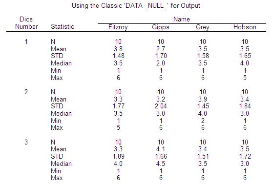
Now lets play with this using a DATA _NULL_ datastep:
          Using the Classic 'DATA _NULL_' for Output

                                       Name
      Dice              ----------------------------------
     Number  Statistic  Fitzroy   Gipps    Grey    Hobson
     -----------------------------------------------------

       1      N          10       10       10       10
              Mean        3.8      2.7      3.5      3.5
              STD         1.48     1.70     1.58     1.65
              Median      3.5      2.0      3.5      4.0
              Min         1        1        1        1
              Max         6        6        6        5

       2      N          10       10       10       10
              Mean        3.3      3.2      3.9      3.4
              STD         1.77     2.04     1.45     1.84
              Median      3.5      3.0      4.0      3.0
              Min         1        1        2        1
              Max         5        6        6        6

       3      N          10       10       10       10
              Mean        3.3      4.1      3.4      3.5
              STD         1.89     1.66     1.51     1.72
              Median      4.0      4.5      3.5      3.0
              Min         1        1        1        1
              Max         6        6        6        6
Just working with this a little more (using some old tricks that I used prior to the existence of PROC REPORT we get the following (output is in RTF format):
HTML output can be easily created using ODS HTML.
Now looking at a graph created using PROC GCHART using the JPEG format:
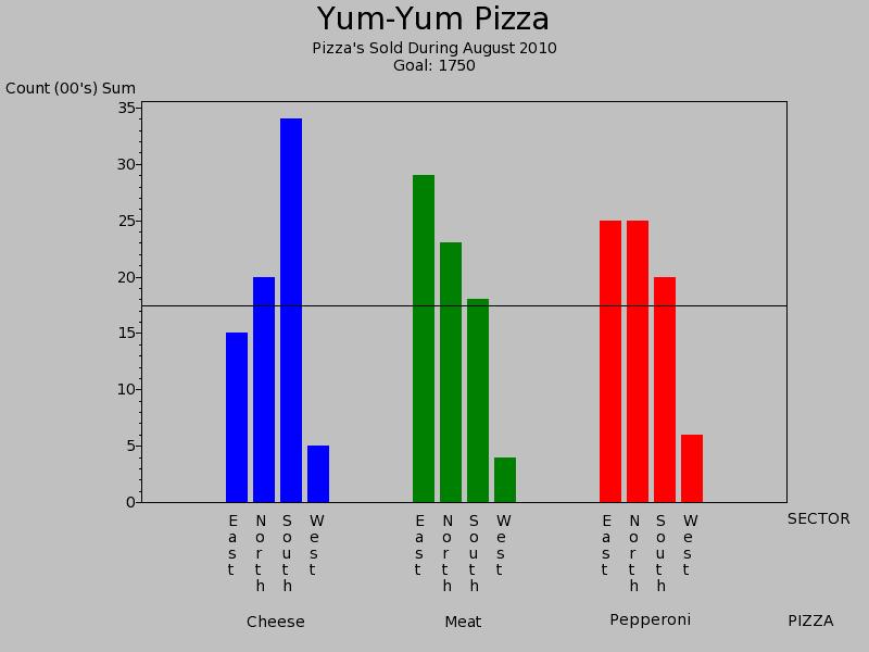
Now an important question, and one that I am always asked when people ask me about WPS -- "where does WPS stack up against SAS?".
The SAS product is large, very large (just a count of the number of Products and Solutions as of this morning was around 268, everywhere from SASŪ for Defense and Aerospace to Banking Solutions, Base SAS to SAS/Toolkit. SAS has been around since the 1970's so their history and product range is extensive.
By contrast WPS has been around since 2000, and has been developing what is now called WPS since 2002.
However, it is unfair to compare the two products this way. If you take the Base SAS, SAS/STAT, SAS/GRAPH and SAS/ACCESS (including engine support) products, against WPS, things get very interesting.
If you consider that WPS has taken the syntax of the SAS language and created its own interpretation with its own interpreter then it is not surprising that there are some features that are not supported that a SAS programmer using the SAS Institute product would expect. Not all the STAT, GRAPH or ACCESS (including Database Support) modules are in WPS, and certainly not all the language is there either, but the more common and regularly used items are there. Yes, there are still features that need to be addressed, but overall WPS has created a product that can take your existing data (maybe it is SAS dataset, Oracle, DB2 or other formats that WPS supports), and use the SAS language to manipulate it, do some statistical analysis and then create output, as the examples above demonstrate.
Any comparison between SAS and WPS must also look at the cost when purchasing the two products. The actual price of SAS or WPS software is dependant on so many factors, including the number of CPUs, but it must be noted that SAS runs around 8 times the price of WPS for the first year, and around 4 times the price thereafter.
World Programming Ltd. has a website that can be found at http://www.teamwpc.co.uk.
October
Using the LABEL and NOOBS options in the PRINT procedure can make your output look better. Refer to the example below:
   === PROGRAM ===
   data reg_cars_US;
	  label year='Year'
	        number='Number of Registered Passenger Cars';
	  format number comma15.;
	  infile cards;
	  input year number comma11.;
	cards;
	2003 135,669,897
	2004 136,430,651
	2005 136,568,083
	2006 135,399,945
	2007 135,932,930
	2008 137,079,843
	;
	proc print data=reg_cars_US;
	   title1 "Listing Without LABEL and NOOBS Options";
	run;
	proc print data=reg_cars_US LABEL NOOBS;
	   title1 "Listing With LABEL Statement";
	run;


   === OUTPUT ===
   Listing Without LABEL and NOOBS Options

        Obs    year             number

         1     2003        135,669,897
         2     2004        136,430,651
         3     2005        136,568,083
         4     2006        135,399,945
         5     2007        135,932,930
         6     2008        137,079,843


         Listing With LABEL Statement

                         Number of
                        Registered
           Year     Passenger Cars

           2003        135,669,897
           2004        136,430,651
           2005        136,568,083
           2006        135,399,945
           2007        135,932,930
           2008        137,079,843
For those who did not notice, the line under the month at the top of the page has a reference to WPS as well as SAS. In an editorial decision, starting this month I will make a reference to whether the tip relates to SAS and WPS, SAS alone, or WPS alone. In the majority of cases the tips will be for both SAS and WPS, but there could be occasions where they relate to one or the other.
See you in November.
November
This month we continue from last month by making a PROC PRINT output look better than just a "data dump", concentrating on the BY and ID options.
Lets look at our program:
   === PROGRAM ===
   ** Our data;
   data SheepNumbers;
      length Country $25 Year Number 8;
      infile cards;
      input Country $ & Year Number;
   cards;
   Australia  2007 85711187
   Australia  2006 91028408
   Australia  2005 101124891
   Canada  2007 879100
   Canada  2006 893800
   Canada  2005 977600
   China  2007 146018203
   China  2006 151337202
   China  2005 152035223
   India  2007 64269000
   India  2006 63558000
   India  2005 62854000
   New Zealand  2007 38460477
   New Zealand  2006 40098191
   New Zealand  2005 39879660
   South Africa  2007 25082100
   South Africa  2006 24982996
   South Africa  2005 25334000
   United Kingdom  2007 33946000
   United Kingdom  2006 34722000
   United Kingdom  2005 35253048
   United States of America  2007 6165000
   United States of America  2006 6230000
   United States of America  2005 6135000
   ;
   run;

   ** Set up standard titles and footnotes;
   title1 "Sheep Numbers in Select Countries, By Year";
   footnote1 "Note: Numbers for India are FAO Estimate";
   footnote2 "Source: UNData, 03Nov2010";

   ** Sort our data for the PRINT procedure. Note use of
      DESCENDING option to sort in decreasing year value.;
   proc sort data=SheepNumbers;
      by Country DESCENDING Year Number;
   run;

   ** Print out a basic lising of the data -- does not
      look very nice, just a "data dump";
   proc print data=SheepNumbers;
      var Country Year Number;
      title2 "(Basic Output)";
   run;

   ** Now something that looks good;
   proc print data=SheepNumbers label;
      by Country;
      id Country;  ** Acts like a "GROUPING" variable;
      var Year Number;
      format Number comma12.;
      label Country='Country'
            Year='Year'
            Number='Repported Number';
      title2 "(A Better Looking Output)";
   run;
The output is:
   === OUTPUT ===
           Sheep Numbers in Select Countries, By Year
                         (Basic Output)

      Obs    Country                     Year      Number

        1    Australia                   2007     85711187
        2    Australia                   2006     91028408
        3    Australia                   2005    101124891
        4    Canada                      2007       879100
        5    Canada                      2006       893800
        6    Canada                      2005       977600
        7    China                       2007    146018203
        8    China                       2006    151337202
        9    China                       2005    152035223
       10    India                       2007     64269000
       11    India                       2006     63558000
       12    India                       2005     62854000
       13    New Zealand                 2007     38460477
       14    New Zealand                 2006     40098191
       15    New Zealand                 2005     39879660
       16    South Africa                2007     25082100
       17    South Africa                2006     24982996
       18    South Africa                2005     25334000
       19    United Kingdom              2007     33946000
       20    United Kingdom              2006     34722000
       21    United Kingdom              2005     35253048
       22    United States of America    2007      6165000
       23    United States of America    2006      6230000
       24    United States of America    2005      6135000

            Note: Numbers for India are FAO Estimate
                   Source: UNData, 03Nov2010
  ------------------------------------------------------------

           Sheep Numbers in Select Countries, By Year
                   (A Better Looking Output)

                                               Repported
                Country             Year          Number

        Australia                   2007      85,711,187
                                    2006      91,028,408
                                    2005     101,124,891

        Canada                      2007         879,100
                                    2006         893,800
                                    2005         977,600

        China                       2007     146,018,203
                                    2006     151,337,202
                                    2005     152,035,223

        India                       2007      64,269,000
                                    2006      63,558,000
                                    2005      62,854,000

        New Zealand                 2007      38,460,477
                                    2006      40,098,191
                                    2005      39,879,660

        South Africa                2007      25,082,100
                                    2006      24,982,996
                                    2005      25,334,000

        United Kingdom              2007      33,946,000
                                    2006      34,722,000
                                    2005      35,253,048

        United States of America    2007       6,165,000
                                    2006       6,230,000
                                    2005       6,135,000

            Note: Numbers for India are FAO Estimate
                   Source: UNData, 03Nov2010
In the second PROC PRINT call, a NOOBS is implied so that option is not required. The variable in the ID statement is used as a "grouping" variable and must also be included in the BY statement -- this is what makes the COUNTRY variable appear as a grouping variable and have a spacing (blank line) between each group. The format COMMA12. is used to make the number appear in comma format so that it is easier to read. As with last month, the LABEL statement and option is used to make user friendly labels appear rather than the variable names. A lot is here so copy the program and try it out.
Will be presenting two papers at NESUG (North East SAS Users Group) conference in Baltimore, Maryland later this month -- if you are there come and say 'hi'.
See you in December.
December
Continuing our series on the PRINT procedure, this month I am looking at the use of the SUM statement, the effect of using the BYLINE option, and creating a basic HTML file. The data that I will be using is automobile numbers by state where the request is for an output of the numbers, but we also want to sum them by a defined region. First I am going to set up a some formats using the FORMAT procedure:
   *----------------------------------------------------------*;
   * Define formats;
   *----------------------------------------------------------*;

   proc format;

     ** Define State abreviation decodes;
     value $statew
       'AL'='Alabama' 'AK'='Alaska' 'AZ'='Arizona' 'AR'='Arkansas'
       'CA'='California' 'CO'='Colorado' 'CT'='Connecticut' 'DE'='Delaware'
       'DC'='District of Columbia' 'FL'='Florida' 'GA'='Georgia' 'HI'='Hawaii'
       'ID'='Idaho' 'IL'='Illinois' 'IN'='Indiana' 'IA'='Iowa' 'KS'='Kansas'
       'KY'='Kentucky' 'LA'='Louisiana' 'ME'='Maine' 'MD'='Maryland'
       'MA'='Massachusetts' 'MI'='Michigan' 'MN'='Minnesota' 'MS'='Mississippi'
       'MO'='Missouri' 'MT'='Montana' 'NE'='Nebraska' 'NV'='Nevada'
       'NH'='New Hampshire' 'NJ'='New Jersey' 'NM'='New Mexico' 'NY'='New York'
       'NC'='North Carolina' 'ND'='North Dakota' 'OH'='Ohio' 'OK'='Oklahoma'
       'OR'='Oregon' 'PA'='Pennsylvania' 'RI'='Rhode Island' 'SC'='South Carolina'
       'SD'='South Dakota' 'TN'='Tennessee' 'TX'='Texas' 'UT'='Utah' 'VT'='Vermont'
       'VA'='Virginia' 'WA'='Washington' 'WV'='West Virginia' 'WI'='Wisconsin'
       'WY'='Wyoming';

     ** Define Regions for Report;
     value $region
       'AK','WA','OR','ID'='Pacific Alaska Region'
       'CA','NV','AZ'='Pacific Region'
       'MT','ND','SD','WY','UT','CO','NM'='Rocky Mountain Region'
       'NE','IA','KS','MO'='Central Plains Region'
       'TX','OK','AR','LA'='Southwest Region'
       'MN','WI','IL','IN','MI','OH'='Great Lakes Region'
       'KY','TN','MS','AL','GA','FL','SC','NC'='South East Region'
       'PA','WV','VA','MD','DC','DE','NJ'='Mid Atlantic Region'
       'NY','VT','NH','CT','RI','MA','ME'='Northeast Region'
       'HI'='Hawaii';
   run;
I have defined a format to decode the state abreviation to the state name, although it is possible to use formats that SAS supplies. Now for some data, shown as a complete data step:
   *----------------------------------------------------------*;
   * Lets bring in our data, Automobile registrations for 2008;
   *----------------------------------------------------------*;

   data cars0;

      ** Lets define the three variables we are going to use;
      attrib state  length=$2 format=$statew. label='State'
             cars   length=8 informat=comma8. format=comma8.
                    label="Number of Automobiles (000's)"
             region length=$25 label='Region';
      infile cards;
      ** First two variables come directly from the data in the CARDS section;
      input state $ cars @@;
      ** Now define REGION from the STATE variable using the format $STATEW
         given above;
      region=put(state,$region.);
   cards;
   AL 2,203 AK 240 AZ 2,217 AR 948 CA 19,706 CO 724 CT 2,007 DE 454 DC 167
   FL 8,064 GA 4,229 HI 480 ID 529 IL 5,704 IN 3,110 IA 1,786 KS 876 KY 1,946
   LA 1,900 ME 555 MD 2,636 MA 3,215 MI 4,337 MN 2,530 MS 1,142 MO 2,613 MT 369
   NE 802 NV 689 NH 646 NJ 3,784 NM 676 NY 8,494 NC 3,539 ND 342 OH 6,345 OK 1,641
   OR 1,433 PA 6,035 RI 486 SC 1,985 SD 343 TN 2,809 TX 8,711 UT 1,180 VT 304
   VA 3,847 WA 3,277 WV 687 WI 2,643 WY 255
   ;
   run;
Our data came in the form of a stream, i.e. not one row per record -- using the '@@' symbol at the end of the INPUT statement tells the input pointer to remain on the current line until all the data for that row is read.
Before we can produce any output we need to set some things up. Along with some options and a footnote that we are going to use on all tables, the data will be sorted by REGION and STATE as the PRINT procedure does not support sorting and we are going to use a BY statement inside the PRINT procedure.
   ** First need to sort the data as PROC PRINT does not sort the data;
   proc sort data=cars0;
      by region state;
   run;

   ** Set some options -- don't put date in the report, and set first page number
      to 1, and set linesize to 64 characters;
   options nodate pageno=1 ls=64;

   ** Set a standard footnote for every output;
   footnote1 "Source: U.S. Department of Transportation, Federal Highway";
   footnote2 "Administration, Highway Statistics 2008 (Washington,";
   footnote3 "DC: 2009), tables MV-1 and MV-9";
Now that we have done the setup, the next job is to produce some output. The first output will be printing the data out by region and state, and summing the number of automobiles in each region, using the BYLINE option:
   === PROGRAM ===
   ** Lets produce the report in classic text form, using the BYLINE option;
   options byline;
   ** LABEL sets option so that dataset variable labels are
      used, UNIFORM sets the column width on each output
      group to be the same, NOOBS switches off printing of
      observation numbers, N sets first the label to use to
      output the number of observations in the group and the
      second label to show the number of observations in the
      entire dataset.;
   proc print data=cars0 label uniform noobs
              n="Number of States in Region: "
                "Total Number of States Analysed: ";
      var state cars;
      by region;
      ** For each region, sum the number of cars as a total at the bottom;
      sum cars;
      ** Now set the title of the report;
      title "Registered Automobiles, 2008";
   run;

   === OUTPUT (PARTIAL) ===
                     Registered Automobiles, 2008                 1

   ----------------- Region=Central Plains Region -----------------

                                            Number of
                                          Automobiles
                 State                        (000's)

                 Iowa                           1,786
                 Kansas                           876
                 Missouri                       2,613
                 Nebraska                         802
                 --------------------    ------------
                 REGION                         6,077

                    Number of States in Region: 4


   ------------------ Region=Great Lakes Region -------------------

                                            Number of
                                          Automobiles
                 State                        (000's)

                 Illinois                       5,704
                 Indiana                        3,110
                 Michigan                       4,337
                 Minnesota                      2,530
                 Ohio                           6,345
                 Wisconsin                      2,643
                 --------------------    ------------
                 REGION                        24,669

                    Number of States in Region: 6


   ------------------------ Region=Hawaii -------------------------

                                            Number of
                                          Automobiles
                 State                        (000's)

                 Hawaii                           480

                    Number of States in Region: 1


   ------------------ Region=Mid Atlantic Region ------------------

                                            Number of
                                          Automobiles
                 State                        (000's)

                 District of Columbia             167


      Source: U.S. Department of Transportation, Federal Highway
         Administration, Highway Statistics 2008 (Washington,
                   DC: 2009), tables MV-1 and MV-9
Using this approach the title is the same but has multiple regions per page.
Another approach is to replace the BYLINE option with a #BYVAL(variable) in the TITLE statement, as the following code will show:
   === PROGRAM ===
   ** Lets produce the report in classic text form without using a BYLINE;
   options nobyline;
   proc print data=cars0 label uniform noobs
              n="Number of States in Region: "
                "Total Number of States Analysed: ";
      var state cars;
      by region;
      sum cars;
      format cars comma8.;
      ** Using a #BYVAL option here so on each page the title will include
         the region name.;
      title "Registered Automobiles for #byval(region), 2008";
   run;

   === OUTPUT (PARTIAL) ===

     Registered Automobiles for Central Plains Region, 2008    5

                                       Number of
                                      Automobiles
              State                     (000's)

              Iowa                        1,786
              Kansas                        876
              Missouri                    2,613
              Nebraska                      802
              --------------------    -----------
              REGION                      6,077

                 Number of States in Region: 4

   Source: U.S. Department of Transportation, Federal Highway
      Administration, Highway Statistics 2008 (Washington,
                DC: 2009), tables MV-1 and MV-9


      Registered Automobiles for Great Lakes Region, 2008      6

                                       Number of
                                      Automobiles
              State                     (000's)

              Illinois                    5,704
              Indiana                     3,110
              Michigan                    4,337
              Minnesota                   2,530
              Ohio                        6,345
              Wisconsin                   2,643
              --------------------    -----------
              REGION                     24,669

                 Number of States in Region: 6

   Source: U.S. Department of Transportation, Federal Highway
      Administration, Highway Statistics 2008 (Washington,
                DC: 2009), tables MV-1 and MV-9


            Registered Automobiles for Hawaii, 2008            7

                                       Number of
                                      Automobiles
              State                     (000's)

              Hawaii                        480

                 Number of States in Region: 1

   Source: U.S. Department of Transportation, Federal Highway
      Administration, Highway Statistics 2008 (Washington,
                DC: 2009), tables MV-1 and MV-9
The output is one region per page, but the title is different because we have included the region name within the title using the #BYVAL statement.
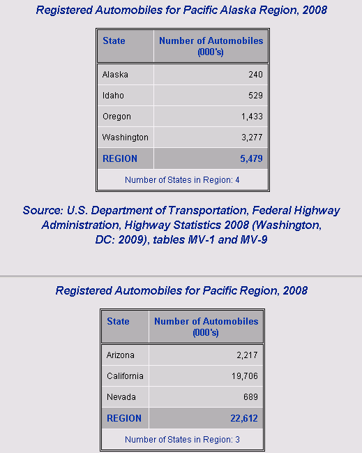
Finally, lets look at what our table looks like on the Web if we produced the output using ODS HTML (default template):
   === PROGRAM ===
   ** Now lets produce the last report in HTML using ODS -- use the same
      code as above but just wrap it with a set of ODS HTML statements.;
   options nobyline;
   ODS html file="C:\TEMP\CARS2008.HTML";
     ** Important, define a location for the output in the first ODS HTML statement;
   proc print data=cars0 label uniform noobs
              n="Number of States in Region: "
                "Total Number of States Analysed: ";
      var state cars;
      by region;
      sum cars;
      format cars comma8.;
      title "Registered Automobiles for #byval(region), 2008";
   run;
   ODS html close;
   run;

   === OUTPUT (PARTIAL) ===
The last three months have been on the PRINT procedure and different ways you can use it to produce output. As you have briefly seen, PRINT can produce nice looking output and do some basic sums and counts of variables when programmed correctly.
Next month it is a new year and a new topic. Have a happy and safe December and see you in 2011!