January
Merging variables from one dataset into another is one of the basic data manipulation tasks that a SAS programmer has to do. The most common way to merge on data is using the MERGE statement in the DATA step but there are three other ways that can help. First though, some data:
    Dataset: PATDATA
    SUBJECT  TRT_CODE
    124263      A
    124264      A
    124266      B

    Dataset: ADVERSE
    SUBJECT  EVENT
    124263   HEADACHE
    124266   FEVER
    124266   NAUSEA
Each of the examples below will merge the TRT_CODE from the PATDATA dataset onto the ADVERSE dataset.
Using the DATA step the code for merging would typically be:
    DATA alldata0;
        MERGE adverse (in=a) patdata (in=b);
        BY subject;
        IF a;
    RUN;
Another way would be to use SQL, so the code would look something like:
    PROC SQL;
        CREATE TABLE alldata0 AS
            SELECT a.*, b.trt_code
            FROM adverse a left join patdata b
            ON a.subject=b.subject;
        QUIT;
    RUN;
A third way is using the KEY= option in the SET statement as shown in the following example:
    DATA alldata0;
        SET adverse;
        SET patdata KEY=subject /UNIQUE;
        IF _IORC_ THEN DO;
            _ERROR_=0;
            trt_code='';
        END;
    RUN;
Before the third example is run the dataset PATDATA must have an index created inside it, using either the INDEX statement inside a DATASETS or SQL procedure, or INDEX option inside a DATA step.
The forth example creates a format from the data and sets the treatment from the created format:
    DATA fmt;
        RETAIN fmtname 'TRT_FMT' type 'C';
        SET patdata;
        RENAME subject=start trt_code=label;
    RUN;
    PROC FORMAT CNTLIN=fmt;
    RUN;
    DATA alldata0;
        SET adverse;
        trt_code=put(subject,$trt_fmt.);
    RUN;
There are other ways of merging data but the above examples show the most common. No one method is better than the other - it depends on the size of the data being merged. The following table gives a guide on the ratio of time spent when compared with a number of observations in the ADVERSE dataset (PATDATA has 1000 patients/records):
     Number of   |   MERGE   |          |             |  PROC
    Observations | Statement | PROC SQL | KEY= Option | FORMAT
    -------------+-----------+----------+-------------+--------
         1K      |    1.00   |    2.19  |     0.25    |   1.25
         1M      |   86.25   |   90.56  |    51.25    |  23.06
         5M      |  787.94   |  402.19  |   302.31    | 264.13
Again, the above table should only be given as a guide. Happy New Year.
February
When the TRIM function is used on a string, the trailing blanks are removed. But did you know that if the string is blank then a single ‘blank’ character is inserted?
But what if we want a ‘null’ string instead?
There is an interesting function called TRIMN that removes trailing blanks from character expressions and returns a null string if the expression is missing.
March
Later this month a series of articles that I have written on Using SAS for Basic Statistics will start appearing on this web site. The first article will deal with Measures of Location and Variance, and how SAS calculates these statistics.
Now for this months' tip. In SAS/SQL it is possible to use the CALCULATED keyword to use values calculated elsewhere in the SQL statment. This prevents the need to recalculate values. The following example avoids having to recalculate the BSAVAL variable for use in the WHERE clause to select patients that have a BSA value of greater than or equal to 2.0:
    PROC SQL;
        SELECT patid, height, weight, SQRT((height*weight)/3600) AS bsaval
            FROM vtialdat
            WHERE CALCULATED bsaval >= 2.0;
        QUIT;
    RUN;
April
Six ways to make your program run faster:
- Use the DROP or KEEP statements to reduce the variables being processed within a DATA step or procedure.
- Use a DATA _NULL_ step when the output from the DATA step is not required.
- Use a CLASS statement rather than the BY statement in a procedure, which may require a SORT first.
- Use the LENGTH statement to minimize variable lengths.
- Create multiple datasets within the one DATA step.
- Where possible, use the WHERE statement in DATA steps and procedures instead of subsetting the data in a DATA step with an IF statement.
May
If a=1, b=. (missing) and c=3, then what does the SAS statement
d = a + b + c;
assign the value for the variable d? The answer is "." or missing as one of the numbers is missing. The correct way of summing the variables and let SAS deal with the missing correctly, i.e. ignore it from the sum, is to use the SAS statement
d = sum(a,b,c);
This last statement will produce the answer of d=4.
June
When people look at SAS code, they will occasionally see the following first line of at datastep:
DATA _NULL_;
This does not create a dataset call _NULL_, but instead runs the datastep without creating a dataset. Why would we want to do this? Not every datastep we run in a SAS program needs to create a dataset - most of the time it will be to get information from a dataset, but there are occasions where some temporary data just needs to be generated for the datastep that is only used for that step. The following example shows an example where we get the number of observations from the dataset SASHELP.CLASS and transfers that number to a macro variable:
   data _null_;
      if 0 then set SASHELP.CLASS nobs=nobs;
      call symput('num',trim(left(put(nobs,8.))));
      stop;
   run;
July
There are three functions that can effect the case of the of text within a character string - LOWCASE, UPCASE and PROPCASE. The following example demonstrates their use:
   22 data _null_;
   23 TextStr="THE COW JUMPED OVER THE MOON";
   24 TextStr_Lower=lowcase(TextStr);
   25 TextStr_Upper=upcase(TextStr);
   26 TextStr_Propper=propcase(TextStr);
   27 put TextStr= /
   28 TextStr_Lower= /
   29 TextStr_Upper= /
   30 TextStr_Propper=;
   31 run;
   TextStr=THE COW JUMPED OVER THE MOON
   TextStr_Lower=the cow jumped over the moon
   TextStr_Upper=THE COW JUMPED OVER THE MOON
   TextStr_Propper=The Cow Jumped Over The Moon
Note how the three functions effected the original text string.
August
Sometimes we need to know if a character variable contains a number, character, or both, or punctuation -- granted, the latter is rare, but it is sometimes still needed. There are a few functions that can help us with this. These are:
ANYALNUM -- Searches a character string for an alphanumeric character
ANYALPHA -- Searches a character string for an alphabetic character
ANYDIGIT -- Searches a character string for a digit
ANYPUNCT -- Searches a character string for a punctuation
In all cases it finds the first character that meets the condition.
The following code demonstrates its use:
   198 data _null_;
   199 TextStr='1313 Mockingbird Lane, Mockingbird Heights';
   200 FirstALNUM=ANYALNUM(TextStr);
   201 FirstALPHA=ANYALPHA(TextStr);
   202 FirstDIGIT=ANYDIGIT(TextStr);
   203 FirstPUNCT=ANYPUNCT(TextStr);
   204 put TextStr= /
   205 FirstALNUM= FirstALPHA= FirstDIGIT= FirstPUNCT=;
   206 run;

   TextStr=1313 Mockingbird Lane, Mockingbird Heights
   FirstALNUM=1 FirstALPHA=6 FirstDIGIT=1 FirstPUNCT=22
September
The last few months have been very busy, finishing off projects for clients, talking a well-deserved break and learning a few new things with SAS and another software package called 'R'. Over the coming months I will pass on some of my new knowledge that I have found useful. Before anyone asks me if I am looking at doing something other than SAS, the answer is no. In my 20 plus years of using SAS I have learnt some of its strengths and weaknesses therefore it is interesting to learn about other software packages and see how they may fill some of the gaps.
This month starts with a very useful SAS option, FORMCHAR. This SAS option sets the characters to be used to build tabular output outlines and dividers for procedures such as the CALENDAR, FREQ, PLOT, REPORT and TABULATE procedures. Its' syntax is:
FORMCHAR = "string";
where the string is a set of 11 characters that set the following:
    Position  Description
    ------------------------
       1      vertical bar
       2      horizontal bar
       3      upper left
       4      upper middle
       5      upper right
       6      middle left
       7      middle middle
       8      middle right
       9      lower left
       10     lower middle
       11     lower right
Positions 3 to 11 are used mainly in drawing boxes. The default string has changed over the years from release to release but a good basic string is
FORMCHAR = "|----|+|---";
The default string can also be set using hex values as the following example illustrates:
FORMCHAR = "82838485868788898A8B8C"x;
October
SAS provides several ways for a user to input data using a CARDS or DATALINES statement. In the examples the CARDS statement is used but the two statements for the most part can be used interchangeably. (The CARDS statement originates from the time when punch cards were used to store data.)
My favorite is known as the List Input, known for its simplicity. The structure for the INPUT statement using this method is to just list the variable names in the order for which the data appears - character variables are specified by using the '$' after the variable name. The following example shows the use of the List Input method where the data being input is the approximate distance from London to certain cities, in kilometers:
    data London2;
        length city $15 distance 8;
        input city $ distance;
        cards;
    Amsterdam 370
    Montreal 5200
    Auckland 22720
    ;
    run;
Note that in all the examples the length of each variable is defined using a LENGTH statement as this overrides any default that SAS may make - for character variables SAS will usually set the length from the value in the first record. (It is good programming practice to define a new variable in a data step with at least a LENGTH statement!)
There is one major problem with the INPUT statement as it is - SAS uses a single space as a delimiter between variables so how could this method be adapted to cater for the name of New York? Two methods exist, the first being the use of the DLM= (delimiter=) option in the INPUT statement as the following example shows:
    data London2;
        length city $15 distance 8;
        infile cards dlm='~';
        input city $ distance;
        cards;
    Paris~330
    New York~5530
    Sydney~215660
    ;
    run;
In the example the character '~' was used but it is possible to use just about any character as a delimiter, popular choices being "," and ";". Note that the DLM option will only work in the INFILE statement. (The INFILE statement is only used in this example as the DLM option is being set, otherwise SAS assumes that the "INFILE CARDS" statement is default from the CARDS statement.)
There is one other adaptation that I personally rarely use and that is to instruct SAS to use a "double space" as a delimiter, as the following example shows:
    data London2;
        length city $15 distance 8;
        input city $ & distance;
        cards;
    Frankfurt  640
    Rio de Janeiro  11060
    Singapore  10810
    ;
    run;
The next best method that I find useful is called the Named Input method which has the feature of allowing the data being input as defined in the INPUT statement to not necessarily be in the same order as in the data after the CARDS or DATALINES statement. The following example will show its use:
    data London2;
        length city $15 distance 8;
        input city= $ distance=;
        cards;
    city=Copenhagen distance=953
    distance=6800 city=Nairobi
    city=Tokyo distance=15260
    ;
    run;
Note that is this method the variable name is followed by the '=' sign in the INPUT and CARDS level.
The third method is the Column method where the columns where the SAS program will find the data is specified in the INPUT statement, as the following example shows:
    data London2;
        length city $15 distance 8;
        input city $ 1-11 distance 13-20;
        cards;
    Rome        1430
    Mexico City 10640
    Hong Kong   13200
    ;
    run;
In the example columns 1 through 11 are reserved for the city name and columns 13-20 are reserved for the distance from London to that city in kilometers.
The last method that data can be input using a CARDS or DATALINES statement is called the Formatted Input method. This is where the INPUT statement has the name of the input variable followed by an informat, as the following example shows:
    data London2;
        length city $15 distance 8;
        input city $11. @13 distance 5.;
        cards;
    Stockholm   1450
    Los Angeles 8780
    Bangkok     12860
    ;
    run;
The last example used what is called a "pointer" (the "@" symbol followed by a number) to instruct the SAS program to go to a particular column and start the input from that column.
It is possible to mix the methods inside an INPUT statement but use caution as unexpected results can easily occur.
I do hope you find this month's tip useful.
November
If you have seperate date and a time variables and you want a single datetime variable combining both, the DHMS function is useful, as the following example demonstrates:
    40    data _null_;
    41        startdate='14Mar2005'd;
    42        starttime='05:15't;
    43        startdatetime=dhms(startdate,0,0,starttime);
    44        put startdate= IS8601DA.
    45            starttime= IS8601TM.
    46            startdatetime= IS8601DT.;
    47    run;
    startdate=2005-03-14 starttime=05:15:00 startdatetime=2005-03-14T05:15:00
Using the DHMS function this way enters the time in seconds as input into the function, which is the same value that SAS stores time from midnight.
I do hope you find this month's tip useful.
December
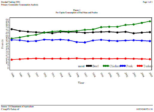
This month will show a method for generating a figure within a RTF document using ODS RTF. Lets first look at the data:
    Consumption of Red Meat and
    Poultry, Per Capita:
    Year Beef Pork Chck Trky
    1988 72.6 52.5 55.0 15.7
    1989 69.3 52.0 57.0 16.6
    1990 67.8 49.8 60.0 17.6
    1991 66.8 50.4 62.0 17.9
    1992 66.5 53.1 66.0 17.8
    1993 65.1 52.4 68.0 17.6
    1994 67.5 53.0 69.0 17.7
    1995 67.0 52.0 68.0 17.7
    1996 67.2 48.4 69.4 18.2
    1997 65.7 47.9 71.4 17.3
    1998 66.7 51.5 72.1 17.7
    1999 67.5 52.7 76.3 17.6
    2000 67.7 51.2 76.9 17.4
    2001 66.4 50.4 76.9 17.6
    2002 67.6 51.5 80.5 17.7
    2003 64.9 51.9 81.5 17.4
    2004 66.1 51.3 84.3 17.1
    2005 67.1 50.3 87.2 16.6
Telling SAS to start an ODS RTF file the following statements are used:
    *Set Directory/Filename for RTF file;
    %let _dirfn=%str(C:\F2-Turkey.rtf);

    *SAS Options;
    options orientation=landscape
            nodate nonumber nobyline;
    run;

    *ODS setup;
    ods listing close;
    ods escapechar '!';
    ods rtf file="&_dirfn"
            style=custom /*Use a customised style*/
            nogtitle nogfootnote;

    *Set GOPTIONS;
    goptions reset=all
             device=png
             target=png
             ftext="Times New Roman"
             xmax=8.95 in ymax=4.25 in;
Now that the setup has been done lets set the titles for the figure:
    title1 j=l "Doodad Trading (NH)"
           j=r "{Page \field{\*\fldinst PAGE}}{ of \field{\*\fldinst NUMPAGES}}";
             /*Sets up Page x of y on right side of first line*/
    title2 j=l "Primary Commodity Consumption Analysis";
    title4 j=c "Figure 1";
    title5 j=c "Per Capita Consumption of Red Meat and Poultry";
    footnote1 j=l '!R"\brdrt\brdrs\brdrw10 "' "Source: US Department of Agriculture";
             /*Set upper boarder of footnote area and footnote 1 text*/
    footnote2 j=l "&_dirfn" j=r "&sysdate9.T&systime";;
             /*Put directory and file name on left side and creation date/time on right*/
Now it is the actual plot of the data:
    *Year axis setup;
    axis1 order=(1988 to 2005 by 1)
          label=(h=1 'Year') value=(h=1 a=-65 r=0)
          offset=(0.1 in) major=(h=0.01 in width=3)
          minor=none width=2;
    *Weight consumption (lbs);
    axis2 order=(0 to 90 by 5)
          label=(h=1.0 a=90 'Pounds')
          value=(h=1.0) length=3.6 in
          minor=none width=2;
    *Set symbols;
    symbol1 value=dot h=1.0 width=3 line=1
            i=join color=black;
    symbol2 value=dot h=1.0 width=3 line=1
            i=join color=green;
    symbol3 value=dot h=1.0 width=3 line=1
            i=join color=blue;
    symbol4 value=dot h=1.0 width=3 line=1
            i=join color=red;
    *Do plot;
    proc gplot data=meat1;
        plot pounds*year=meat
             /haxis=axis1
              vaxis=axis2
              legend=legend1;
        legend1 POSITION=(BOTTOM
                          RIGHT
                          INSIDE);
    run;
    quit;
The final output looks like the following:
I do hope you find this month's tip useful. Merry Christmas.